Two papers from DeepSeek bracket the company’s 2025 work on long-context attention: Native Sparse Attention (NSA) in February (arXiv:2502.11089) and DeepSeek Sparse Attention (DSA) shipped inside DeepSeek-V3.2 in December (arXiv:2512.02556). Both attack the same problem — full attention is and unaffordable at the context lengths frontier models now serve — but they reach surprisingly different designs. NSA is a parallel three-branch mechanism trained from scratch. DSA is a single-branch top- selector bolted onto an already-trained dense model.
This post walks the math of both, then explains why DSA looks the way it does given that NSA came first.
Table of contents
Open Table of contents
Why sparse attention, and why “native”?
Standard softmax attention computes, for each query over the prefix :
The cost is in both compute and KV traffic. At this dominates the forward pass; at the KV cache itself becomes a memory-bandwidth problem during decode.
Decade-old observation: the attention matrix is empirically sparse — most queries attend non-trivially to a small subset of keys. The natural response is to skip the negligible entries. The trap is that most “skip” strategies (post-hoc pruning, hashing, fixed local+global patterns) are either:
- Not trainable end-to-end — you sparsify a dense-trained model at inference, and the model never learned to live with the sparsity, so quality drops.
- Not hardware-aligned — the irregular index patterns wreck GPU memory coalescing, so the theoretical FLOP savings don’t materialize as wallclock speedup.
NSA’s contribution is in the name: natively trainable (the sparse pattern is learned during pretraining) and hardware-aligned (the selection unit is a contiguous block, sized to match GPU memory transactions). DSA inherits the same two commitments but reshapes them around a different deployment story.
Part 1 — Native Sparse Attention (NSA)
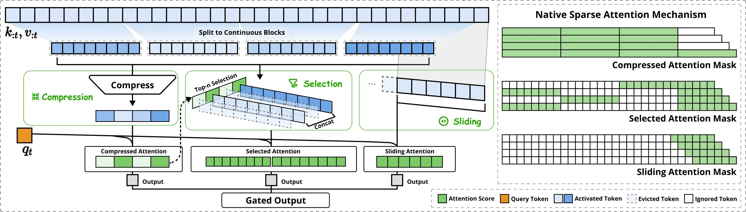
Figure 2 from Yuan et al. (2025), arXiv:2502.11089. Left: the three parallel branches — compressed attention for coarse global context, selected attention for important token blocks, sliding attention for local context. Right: the corresponding attention patterns; green = computed, white = skipped.
The three-branch decomposition
NSA replaces the single attention operator with three parallel branches whose outputs are combined by learned gates:
Each branch defines its own remapped key/value set . The gates are produced by a small MLP from the hidden state. The three branches are:
- cmp — coarse attention over a small number of compressed block-summaries (covers the whole prefix).
- slc — fine attention over a handful of full-resolution token blocks selected per query (covers the important regions).
- win — local sliding-window attention over the last tokens (covers recent context).
The crucial design choice is that the three branches use independent K/V, not a shared set with three masks. The paper argues that a shared K/V would let the easy local-window gradients dominate, preventing the compressed/selected branches from ever learning to do useful work.
Branch 1: compressed (cmp)
Partition the prefix into overlapping blocks of length with stride (defaults , ). A learned MLP — with intra-block positional encoding — compresses each block of key vectors into a single summary key:
An identical (different weights) produces . So instead of attending to keys, the compressed branch attends to roughly summary tokens — a ~16× reduction. This branch is cheap and globally aware, but lossy.
Branch 2: selected (slc)
This is where the cleverness lives. We want each query to fetch a few full-resolution blocks where the action actually is. How do we pick them without spending per query?
NSA reuses the compressed-branch attention as a free block importance score. After the cmp branch computes its softmax,
we have one scalar score per compressed block. With a small fixup (because the compression block size and the selection block size — default — may differ, the cmp-block scores are aggregated/redistributed onto slc-block boundaries; and across a GQA group the per-head scores are summed so all heads in a group select the same blocks), we obtain a per-slc-block score . Then top-:
Defaults: selected blocks per query, but with two reservations — 1 block fixed at the very start of the sequence (the “attention sink”) and 2 blocks fixed at the local end. So 13 are dynamically chosen by the importance score and 3 are fixed.
Two consequences worth highlighting:
- The selector is differentiable upstream. The block scores come from a softmax that participates in the loss, so gradients flow back through the importance-scoring path even though top- itself is non-differentiable. The selection which is hard; the whether-to-trust-this-score is soft.
- Per-GQA-group selection is mandatory for kernels. If each query head in a group picked its own blocks, the kernel would have to issue different KV loads per head, killing the bandwidth savings that GQA exists for. NSA aggregates scores across heads in a group so the whole group shares one . That single decision is what makes the speedups real.
Branch 3: sliding window (win)
Just the trailing tokens (default ): . Cheap, dense, and absorbs the easy local-attention gradient that would otherwise corrupt the other two branches’ learning.
Hardware alignment — why blocks, not tokens
Per-token top- selection produces an unsorted scatter of indices, and a Flash-Attention-style kernel cannot stream contiguous KV tiles from HBM into SRAM if the indices look like [7, 412, 1188, ...]. NSA’s selection unit is a block of contiguous tokens, chosen so that the SRAM tile size satisfies . Concretely, the NSA kernel:
- Group-centric query loading. Loads all query heads of a GQA group at position together, , since they share .
- Shared KV fetching. Streams the selected blocks once into SRAM and amortizes them across all heads in the group.
- Triton grid scheduling. Balances arithmetic intensity so the kernel is compute-bound, not bandwidth-bound, even at moderate block counts.
The reported wallclock numbers at 64k context: ~9.0× forward, ~6.0× backward, ~11.6× decode vs dense Flash-Attention. The decode number is largest because decoding is memory-bound and the reduction in KV traffic is the most direct lever there.
NSA in one picture
For each query you spend:
- attention ops on compressed summaries (always),
- attention ops on selected full-res blocks (default ),
- attention ops on the sliding window (default ),
for a total of roughly effective KV reads per query — additive in for the compressed branch and constant in for the other two. The model used in the paper is 27B params (3B active MoE), 30 layers, , , GQA with 4 groups / 64 heads, pretrained on 270B tokens at 8k length then continued at 32k with YaRN.
Part 2 — DeepSeek Sparse Attention (DSA) in V3.2
NSA was published in February. By December, DeepSeek shipped V3.2 with a different sparse mechanism. Why?
The honest answer is mostly pragmatic. V3 / V3.1-Terminus already exists as a several-hundred-billion-parameter dense-attention MoE that cost a fortune to train. You cannot re-architect its attention into three branches and continue training cheaply — the model has already shaped its representations around the dense operator. DSA is a minimally invasive sparsifier: it keeps the existing attention block almost intact and adds a cheap external selector.
The lightning indexer
DSA’s core trick is to factor sparsity out of the attention block. Instead of deriving importance scores from attention (as NSA does via the cmp branch), DSA computes them with a separate, dramatically cheaper module — the lightning indexer. For each query position and prefix position :
Read this carefully:
- is a small number of indexer heads (much smaller than the main attention’s head count).
- are separate, low-dimensional projections of the hidden states — not the main attention’s Q/K.
- is a per-token, per-head scalar weight (a tiny linear from ).
- The activation is ReLU, not softmax. Two reasons: (i) ReLU is much faster than on tensor cores; (ii) the indexer doesn’t need to be a probability distribution — it just needs to rank.
- The entire indexer is designed to run in FP8. At low precision, with ReLU and few heads, the per-pair cost is tiny.
The indexer is still in pair count, but its constant factor is so small that the paper reports it costs much less than the main MLA attention in V3.1-Terminus.
Top-k selection and the main attention
Given the index scores, DSA picks the top- keys per query and runs the main attention only over those:
Two design choices matter:
- is per-token, not per-block. Unlike NSA’s blockwise selection, DSA selects individual tokens. The blocking that NSA needed for kernel efficiency is recovered in a different way — through MLA, see below.
- DSA piggybacks on MLA’s MQA mode. V3 already uses Multi-head Latent Attention; in MLA the K/V cache is a single shared latent per token rather than per-head K/V projections. So when DSA selects a token, all query heads share the same latent vector — exactly the GQA-style amortization NSA had to engineer manually. This is the architectural reason DSA can afford per-token (rather than per-block) selection.
The main attention’s complexity drops from to with . At , that is a ~64× reduction in main-attention FLOPs.
Two-stage training: KL distillation from a frozen teacher
DSA must not regress the existing model. The training recipe is the most interesting part of the paper and consists of two stages:
Stage A — dense warm-up (indexer only). Freeze the entire base model. The main attention still runs dense, producing a reference attention distribution. Aggregate the dense attention scores across all query heads and L1-normalize to obtain a per-token target distribution . Train only the indexer with a KL objective:
That is: teach the indexer to mimic, in score-space, what dense attention attends to. Recipe: 1,000 steps, ~2.1B tokens, lr . The base model never updates during this stage.
Stage B — sparse training (everything). Switch the main attention to top- sparse mode and unfreeze the base model. The KL loss is restricted to the selected positions :
and the indexer’s input is detached from the main computational graph, so the indexer is optimized purely by while the base model is optimized purely by the language-modeling loss. Recipe: 15,000 steps, ~943.7B tokens, lr .
In other words: Stage A makes the indexer a competent imitator of dense attention; Stage B lets the base model gracefully adapt to consuming only the indexer’s top- picks, while the indexer keeps refining its imitation on the support it actually picks. Per the paper, V3.2-Exp ends up at parity with V3.1-Terminus on short and long-context evals — with a much cheaper attention at inference.
Part 3 — NSA vs DSA, side by side
The two designs share a worldview (sparsity should be learned and hardware-friendly) but answer four design questions differently:
| Question | NSA | DSA |
|---|---|---|
| Where do importance scores come from? | Compressed-branch attention (reused softmax) | Separate lightning indexer (ReLU, FP8) |
| Selection granularity | Blocks of tokens | Individual tokens, |
| How are GQA heads amortized? | Per-group block selection in kernel | Inherited from MLA’s latent K/V |
| When is sparsity learned? | Pretrained natively from scratch | Bolted on via 2-stage continued training |
| What does the rest of the model see? | Three parallel attention branches with gating | A single attention branch, mostly unchanged |
A useful way to phrase the difference: NSA designs sparsity into the architecture. DSA designs sparsity onto the architecture. NSA pays the cost up front (re-pretraining) and gets a richer, multi-resolution attention. DSA pays the cost at the end (continued training) and gets a much smaller diff against an existing dense model — important when the dense model is V3-scale and you cannot afford to throw it away.
There is also a quieter point: DSA’s reliance on MLA is what makes its per-token selection viable. NSA’s blockwise selection is partly a workaround for not having a shared-latent K/V — it forces locality at the granularity where GPU kernels are happy. Once you have MLA, the block constraint relaxes and you can be more surgical. This is a nice example of how lower-level architectural choices (the K/V representation) propagate into upper-level algorithmic ones (how you sparsify).
Part 4 — What’s actually doing the work
A few things stand out across both papers that are worth internalizing beyond the specific designs:
- The hard part of “sparse attention” is not the sparsity, it’s the gradient. Top- is not differentiable. NSA threads gradients through the scoring softmax even though the selection itself is not. DSA sidesteps the problem entirely by training the indexer with an external KL target derived from a frozen dense teacher. Both are valid; neither is the obvious thing.
- Hardware co-design is non-negotiable. Both papers spend disproportionate space on memory layout, block size constraints, and kernel scheduling. A sparse pattern that doesn’t translate into contiguous KV tiles is, in practice, slower than dense Flash-Attention.
- MLA changed the design space. Many of the choices in DSA — per-token selection, the small index head dimension, the cheap indexer — are downstream of having a single shared latent per K/V. If you’re designing a long-context attention mechanism in 2026, the K/V cache representation is upstream of the sparsity strategy, not orthogonal to it.
- Continued-training recipes are a first-class research artifact now. The two-stage KL recipe in DSA is the kind of thing that, five years ago, would have been a footnote. It is now the entire point of the paper — because at frontier-model scale, how you modify a trained model matters as much as what you modify.
Closing
NSA and DSA are best read together. NSA shows what sparse attention looks like when you have the freedom to design it from scratch; DSA shows what it looks like when you don’t, and have to graft it onto a model that the world is already using. The fact that DeepSeek shipped both within a year — and that DSA does not simply inherit NSA — is itself the most interesting signal: the right sparsity story depends on the constraints of the model you are training, not just on the asymptotics.
References
- Yuan, J. et al. Native Sparse Attention: Hardware-Aligned and Natively Trainable Sparse Attention. arXiv:2502.11089, 2025.
- DeepSeek-AI. DeepSeek-V3.2: Pushing the Frontier of Open Large Language Models. arXiv:2512.02556, 2025.