DeepSeek just open-sourced DeepSpec — “a full-stack codebase for training and evaluating draft models for speculative decoding” — and with it a paper on its headline algorithm, DSpark (Cheng et al., a Peking University × DeepSeek-AI collaboration). DSpark is the speculative-decoding stack that runs in production behind the preview DeepSeek-V4-Flash and DeepSeek-V4-Pro models, where it replaced the previous single-token drafter two weeks after the V4 preview shipped.
The one-sentence version: DSpark makes the draft model draft better (a semi-autoregressive drafter that fixes the quality problem of parallel draft heads) and makes the target model verify smarter (a confidence-scheduled, load-aware verifier that stops wasting compute on tokens that are going to be rejected). Against DeepSeek’s own MTP-1 production baseline, that combination buys 60–85% faster per-user generation at matched throughput.
This post walks the whole thing: a recap of how speculative decoding works, a tour of the drafter design space (vanilla speculative decoding, Medusa, EAGLE, MTP, and parallel drafters like DFlash), what exactly DSpark adds on top, the math, and the production numbers.
Table of contents
Open Table of contents
- The setting: why decoding is slow
- The drafter design space (and where the prior work sits)
- What DSpark actually is
- Idea 1: semi-autoregressive generation
- Why can parallel generation beat autoregression at all?
- Idea 2: confidence-scheduled verification
- Training
- Results: offline draft quality
- Results: production deployment in DeepSeek-V4
- How DSpark compares, at a glance
- Limitations and takeaways
The setting: why decoding is slow
LLMs generate autoregressively — every new token needs a full forward pass conditioned on all preceding tokens — so latency scales with output length, GPU utilization is low (one token’s worth of compute per memory-bandwidth-bound pass), and the user waits. For latency-sensitive products (chat assistants, multi-turn agents) this is the bottleneck.
Speculative decoding (Leviathan et al., 2023; Chen et al., 2023) is the standard fix. A lightweight draft model proposes a block of candidate tokens . The full-size target model then verifies the entire block in a single forward pass, accepting the longest prefix consistent with its own distribution and appending one bonus token.
The verification rule is what makes this lossless. At draft position the target computes its own distribution and accepts the draft token with probability
Verification proceeds left to right; the first rejection at position discards every token after it. On a rejection the target resamples from the residual , so the output is distributed exactly as if the target had decoded on its own — speculative decoding accelerates generation with zero quality loss.
Let be the number of accepted tokens per cycle and , the wall-clock times of the two passes. The average latency per generated token is
Every speculative-decoding paper is, at bottom, pulling one of three levers in this equation: draft faster (lower ), draft better (raise ), or verify smarter (cut the effective ). DSpark is unusual in that it pulls two of them at once.
The drafter design space (and where the prior work sits)
The whole game is the draft model: its architecture decides how and trade off. Historically there have been two camps.
Autoregressive drafters — high \tau, but T_{\text{draft}} \propto \gamma
The earliest drafters are themselves small autoregressive models, conditioning each draft position on the previously sampled draft tokens.
- Vanilla speculative decoding uses a separate, smaller LM from the same family as the draft. It drafts well but you have to have a well-aligned small model, and the draft is sequential.
- EAGLE / EAGLE-2 / EAGLE-3 (Li et al.) move the autoregression into feature space: a small head autoregressively predicts the target’s next hidden feature, reusing the target’s own embedding and LM head, and expands candidates into a dynamic draft tree. EAGLE-3 drops the feature-regression constraint and trains directly on the target’s outputs (“training-time test”). It is the strongest autoregressive drafter and serves as DSpark’s AR baseline.
- MTP (Multi-Token Prediction), from the DeepSeek-V3 report, bolts sequential MTP transformer modules onto the target itself, each conditioning on the previous module’s output. This is what DeepSeek actually ran in production — as MTP-1, a single extra token.
The common wall: because generation is sequential, drafting cost grows with block size, . To keep small you are forced into shallow heads and short blocks. Tree-based verification (SpecInfer) widens the candidate set but spends more verification tokens to do it.
Parallel drafters — T_{\text{draft}} is flat, but \tau decays
The other camp produces all draft tokens in a single forward pass, so is nearly independent of block size and you can afford a deep drafter and a large block ( is cheap).
- Medusa (Cai et al., 2024) attaches extra decoding heads to the target’s final hidden state; head predicts the token positions ahead. All heads fire in parallel, and a tree-attention pass verifies combinations.
- DFlash (Chen et al., 2026) is the current state-of-the-art parallel drafter and the one DSpark builds on. It is diffusion-inspired: the drafter takes an anchor token plus mask tokens and decodes all positions at once, conditioned on rich target context injected as extra keys/values. Concretely, hidden states from a set of target layers are projected into the draft space,
and concatenated onto every draft layer’s keys and values, , , so all block positions attend bidirectionally to each other and to the target context.
The structural problem with every parallel drafter is independence. Because each position is predicted in one shot, it cannot condition on what the other positions actually sampled. When the context admits two plausible continuations — say “of course” and “no problem” — a parallel drafter marginalizes over both and happily emits the incoherent cross-products “of problem” or “no course.” This is the classic multi-modal collision of non-autoregressive generation, and it makes acceptance decay rapidly along the block.
So you are stuck choosing between an autoregressive drafter that models dependencies but can’t scale its depth or block size, and a parallel drafter that scales beautifully but proposes incoherent suffixes. DSpark’s first contribution is to refuse the choice.
What DSpark actually is
DSpark is two complementary mechanisms layered onto a parallel drafter:
- Semi-autoregressive generation. Keep the heavy, high-capacity draft backbone fully parallel (so stays flat in ), then append a lightweight sequential head that injects local token-to-token dependency. You recover most of an autoregressive drafter’s coherence at almost none of its latency cost.
- Confidence-scheduled verification. Attach a calibrated confidence head that predicts each draft token’s survival probability, and a hardware-aware scheduler that uses those probabilities — together with the engine’s real-time throughput profile — to decide, per request, how many tokens are actually worth verifying.
Here is the full decoding cycle.

Figure 1 from Cheng et al., DSpark (2026). Given ABC, the target emits anchor D. DSpark’s parallel backbone + sequential head draft EFGH with confidence scores; the scheduler keeps EFG and drops the low-confidence H; the target verifies in parallel, accepting E,F, rejecting G, and generating the corrected bonus token G*.
The rest of the post unpacks the two halves.
Idea 1: semi-autoregressive generation
DSpark splits drafting into a parallel stage and a sequential stage.
Parallel stage. A DFlash backbone runs a single forward pass over the whole block, producing hidden states and base logits . (DSpark makes one small change to DFlash: it treats the anchor token itself as the first prediction position, so input tokens — anchor plus masks — yield draft logits, shaving a bit of draft compute.)
Sequential stage. This is the new piece. Instead of using the base logits directly, DSpark adds a prefix-dependent transition bias that lets each position condition on the tokens already sampled earlier in the same block. Crucially, rather than defining a globally normalized energy model, it induces a proper causal factorization:
where is the anchor token and is the vocabulary. At inference the sequential block samples left to right.
This locality is the subtle, important design choice. Because each is an exact, locally normalized softmax, DSpark can hand the target an exact per-token probability — which is precisely what the rejection-sampling rule needs. This is why DSpark stays lossless where structured-output non-autoregressive layers cannot: a CRF drafter’s globally normalized partition function and a CTC drafter’s marginalization over alignments both destroy exact per-token probabilities, forcing them into greedy-only verification. DSpark keeps the sequential correction local, so per-token probabilities remain plain softmax evaluations.
Because the sequential loop is inherently serial, it has to be cheap enough that . DSpark offers two instantiations:
- Markov head (default). depends only on the immediately preceding token, a first-order transition . A full table would be enormous, so it is factorized low-rank, with , and . Given , the bias for position is just an embedding lookup followed by a projection, . Back to the example: once position 1 samples “of”, the Markov head boosts “course” and suppresses “problem” at position 2 — collision averted.
- RNN head. The Markov head is memoryless beyond one step; the RNN head carries a recurrent state that accumulates the full in-block prefix. It concatenates and applies a single gated update. It does a little better at long block lengths, but at higher implementation cost — so DSpark ships the Markov head.
A little autoregression goes a long way
How much does this lightweight head actually help, and what does it cost? Two clean results from the paper:
- Parameter efficiency. With block size fixed, a 2-layer DSpark beats a 5-layer DFlash baseline across math, code, and chat. Injecting local autoregression is a far better use of parameters than stacking more parallel depth.
- Negligible latency. Scaling the draft length from 4 to 16 tokens adds only 0.2%–1.3% to full-round latency over DFlash, because at production batch sizes the target’s verification pass dominates and the serial sampling loop disappears into the noise. The payoff for that rounding error is up to a 30% longer accepted length.
Why can parallel generation beat autoregression at all?
Here is the counter-intuitive headline from the offline results (full table below): the parallel DFlash and semi-autoregressive DSpark both produce longer accepted lengths than the fully autoregressive EAGLE-3 — even though conventional wisdom says step-by-step autoregression yields higher-quality sequences. The paper explains this with a position-wise conditional acceptance metric: for each position , it measures the acceptance rate given that all earlier tokens were already accepted, isolating the predictive quality at that step from the penalty of earlier rejections.
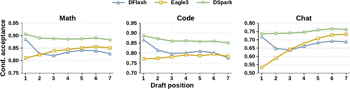
Figure 2 from Cheng et al., DSpark (2026). Conditional acceptance per draft position (Qwen3-4B). The autoregressive drafter (EAGLE-3) is stable or rising; the parallel drafter (DFlash) suffers suffix decay; DSpark stays high and stable throughout.
The curves tell a two-part story:
- Position 1 — the capacity advantage. At the very first draft position, every architecture predicts from the same target context, so the gap is pure model capacity. Autoregressive EAGLE-3 is forced shallow by its latency budget; the parallel drafters are and can be deep. That deeper network wins position 1 outright (e.g., 0.88 vs 0.81 on math, 0.72 vs 0.53 on chat). And because verification is a strict left-to-right prefix match, the first token carries the most leverage — a rejection there throws away the whole block. So a position-1 edge is worth far more than its single token, which is why parallel drafters win globally despite decaying later.
- Positions 2–7 — the independence tax. Down the tail, DFlash decays (0.87 → 0.78 on code, 0.72 → 0.63 on chat) exactly as multi-modal collision predicts, while autoregressive EAGLE-3 actually climbs (0.53 → 0.74 on chat) as the locked-in prefix makes later tokens more predictable.
DSpark gets both: it inherits the deep parallel backbone’s high position-1 acceptance (starting around 0.93 on math) and uses the sequential head to kill the decay, staying high and flat across the whole block. That is the entire argument for semi-autoregression in one figure.
Idea 2: confidence-scheduled verification
A good drafter that proposes long blocks is necessary but not sufficient. Verifying more tokens does not automatically mean faster generation, because the value of verifying an extra token depends on two things:
- Data. Structured tasks (code, math) sustain high acceptance deep into the block; open-ended chat does not. A fixed verification length wastes compute on chat’s doomed trailing tokens.
- System load. Under light load, verifying a few extra tokens is nearly free. Under high concurrency, every speculative token you verify occupies target-model batch capacity that could have served another user’s request. Past a point, over-eager verification actively lowers total throughput.
DeepSeek had been feeling exactly this in production: deploying a static multi-token drafter (MTP-3/5) degraded aggregate throughput under load, which is why they conservatively shipped single-token MTP-1. DSpark’s second half is the mechanism that makes long draft blocks safe to deploy.
The confidence head
For each draft position , a tiny linear-plus-sigmoid head predicts a survival probability — the chance token survives verification given that all earlier tokens were accepted:
It is supervised against the analytical per-step acceptance rate, which (from the rejection-sampling rule) is one minus half the total-variation distance between draft and target distributions:
Calibration matters: Sequential Temperature Scaling
Most prior “adaptive draft length” heuristics only need confidence scores to rank tokens correctly. DSpark’s scheduler needs more: it has to compute an expected accepted length, so it needs the absolute magnitudes of the cumulative survival probabilities to be right. Neural confidence estimates are notoriously overconfident, which would distort the throughput math.
The fix is Sequential Temperature Scaling (STS). Since each is a conditional probability, the joint probability that a prefix of length survives is the cumulative product . STS calibrates this product left to right: at each position it does a 1-D grid search for the temperature that minimizes the Expected Calibration Error of the cumulative product, holding earlier positions fixed. Because temperature scaling is order-preserving, it fixes the probabilities without disturbing the rankings the head learned. On Alpaca this pulls the head’s calibration error from a 3–8% range down to roughly 1%, while discrimination stays strong (ROC-AUC 0.81–0.90).
The hardware-aware prefix scheduler
Now the payoff. Consider a batch of active requests. For request , the survival probability of its prefix up to position is the cumulative product . If we verify tokens for each request, the total verification batch (in tokens) is and the expected number of accepted tokens is
Let be the engine’s throughput (forward steps per second) at batch size — a capacity curve profiled once at startup and stored as a lookup table. The scheduler picks the per-request verification lengths that maximize system-wide token throughput:
This looks combinatorial, but it has a clean greedy solution. The marginal gain from extending request from to verified tokens is exactly , and survival probabilities are monotonically non-increasing along a block (). So you can simply sort all candidate prefix-extensions across all requests in descending order of survival probability and admit them one at a time, each update an lookup into the cost table — stopping when stops improving.
That early-stop is not just an optimization; it is what keeps the whole thing lossless. Lossless speculative decoding requires the non-anticipating property: the decision to admit token must not depend on the realization of token itself. But the Markov confidence head computes using the sampled token , so a retrospective global search would leak future tokens into earlier admission decisions and quietly bias the output distribution.
The bias is real, and the paper proves it. In a worked single-request example with and : a global search that peeks at admits the first token only when happens to lead to a confident continuation. Carried through the rejection-sampling algebra, the output token comes out distributed instead of the target’s true — not lossless. Breaking the greedy loop the instant throughput drops isolates the admission decision from future tokens and restores exactness.
How aggressive is this pruning? A static threshold sweep gives the intuition: pushing the confidence threshold up drives chat’s acceptance rate from 45.7% all the way to 95.7% (chat has the most doomed trailing tokens to cut), while structured code and math — which were already healthy — climb more gently (67.6% → 92.0% and 76.9% → 92.5%). The scheduler is essentially a load-aware version of that knob, turned automatically per request.
Training
The drafter is trained with the target model frozen and its embedding + LM head shared and frozen; only the backbone, sequential block, and confidence head update. Three losses, each position-weighted by to emphasize the high-leverage early positions:
The interesting one is . Since per-step acceptance is , total-variation distance is a direct proxy for acceptance — minimizing it is maximizing expected acceptance, which is why it dominates the weighting (0.9) over plain cross-entropy (0.1). The confidence loss is a binary cross-entropy training the head to predict the soft acceptance label .
Results: offline draft quality
With the scheduler disabled (everyone proposes a fixed block) so we see raw draft quality, here is accepted length per decoding round across four target models and three domains. Higher is better; bold is best.
| Target | Drafter | GSM8K | MATH | AIME25 | MBPP | HumanEval | LCB | MT-Bench | Alpaca | Arena-Hard |
|---|---|---|---|---|---|---|---|---|---|---|
| Qwen3-4B | EAGLE-3 | 5.14 | 4.62 | 3.92 | 3.69 | 4.16 | 3.77 | 2.39 | 2.26 | 2.55 |
| DFlash | 5.40 | 4.85 | 4.15 | 4.40 | 4.74 | 4.18 | 3.07 | 2.96 | 2.83 | |
| DSpark | 6.11 | 5.70 | 4.89 | 5.13 | 5.38 | 4.86 | 3.64 | 3.54 | 3.29 | |
| Qwen3-8B | EAGLE-3 | 5.30 | 4.77 | 3.91 | 3.96 | 4.33 | 4.17 | 2.66 | 2.54 | 2.54 |
| DFlash | 5.33 | 4.91 | 4.07 | 4.36 | 4.64 | 4.39 | 3.11 | 2.98 | 2.81 | |
| DSpark | 6.17 | 5.78 | 5.01 | 5.16 | 5.52 | 5.17 | 3.72 | 3.58 | 3.21 | |
| Qwen3-14B | EAGLE-3 | 5.24 | 4.60 | 3.71 | 3.81 | 4.14 | 4.01 | 2.62 | 2.47 | 2.48 |
| DFlash | 5.41 | 4.84 | 3.98 | 4.44 | 4.59 | 4.33 | 3.10 | 2.94 | 2.72 | |
| DSpark | 6.21 | 5.74 | 4.94 | 5.26 | 5.43 | 5.02 | 3.70 | 3.58 | 3.13 | |
| Gemma4-12B | EAGLE-3 | 5.87 | 5.46 | 4.83 | 4.72 | 5.37 | 4.16 | 3.19 | 3.06 | 2.72 |
| DFlash | 5.45 | 5.04 | 4.22 | 4.39 | 4.95 | 3.70 | 2.98 | 2.84 | 2.59 | |
| DSpark | 6.05 | 5.78 | 5.12 | 5.11 | 5.64 | 4.51 | 3.49 | 3.35 | 2.92 |
DSpark wins every cell. In macro-average accepted length it beats the autoregressive EAGLE-3 by 30.9% / 26.7% / 30.0% on Qwen3-4B/8B/14B, and the parallel DFlash by 16.3% / 18.4% / 18.3% — and the gains carry across model families (Gemma4-12B). The strong domain effect is also visible: accepted length is naturally high on structured tasks (~5+ on math and code) and low on open-ended chat (~3.5), which is exactly the variance the confidence scheduler exists to exploit.
Results: production deployment in DeepSeek-V4
Offline accepted length is the algorithm; the real test is live traffic. In production DSpark is configured as DSpark-5 (): a parallel backbone of three MoE layers with mHC and a sliding window of 128, the Markov head, and the STS-calibrated confidence head. Getting there required real systems work — training-side, communicating only pre-LM-head hidden states to cut per-token communication to , and packing isolated draft anchors via token-level attention indices; inference-side, an asynchronous scheduler that estimates capacity from confidence outputs two steps prior (so it composes with CUDA-graph replay and zero-overhead scheduling) and flattened variable-length kernels so the dynamic per-request verification lengths don’t wreck GPU utilization.
The headline comparison is against MTP-1, the single-token drafter DSpark superseded in production.
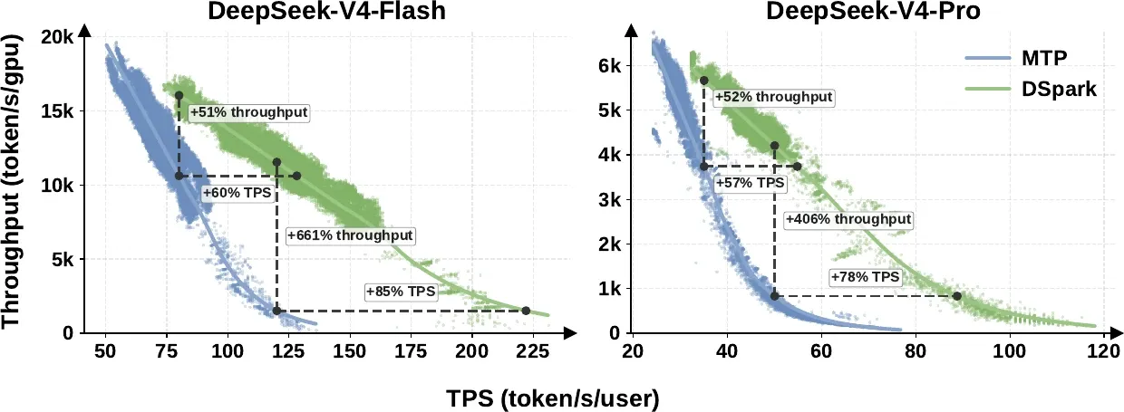
Figure 7 from Cheng et al., DSpark (2026). Aggregate throughput vs per-user generation speed (TPS) under live traffic. DSpark pushes the throughput–interactivity Pareto frontier outward relative to the MTP-1 baseline.
Reading the frontier with SLA = the minimum per-user speed the system must guarantee:
- At matched throughput, DSpark delivers 60–85% faster per-user generation on V4-Flash and 57–78% faster on V4-Pro.
- At a moderate SLA (80 tok/s/user on Flash, 35 on Pro), it lifts aggregate throughput by ~51–52%.
- At a strict SLA (120 on Flash, 50 on Pro), the single-token baseline is up against its operational wall and can sustain only a tiny batch — so DSpark’s nominal throughput advantage balloons to 661% / 406%. The authors are careful (and correct) to read these as evidence that DSpark unlocks interactivity tiers the baseline simply cannot serve, not as a representative multiplier over a well-utilized system.
The mechanism behind the frontier shift is the load-adaptive scheduler doing its job:
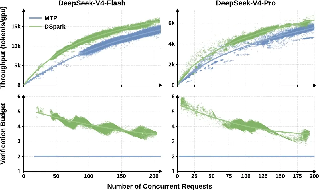
Figure 8 from Cheng et al., DSpark (2026). DSpark’s per-request verification budget expands to ~4–6 tokens when target compute is idle and contracts smoothly as concurrency saturates the target — versus MTP-1’s static 2 tokens.
Where MTP-1 verifies a flat 2 tokens regardless of load, DSpark spends 4–6 tokens per request when the target has idle capacity and smoothly tightens the budget as concurrency rises, pruning low-confidence tokens before they steal batch capacity. That is what converts longer draft blocks into a frontier shift instead of a throughput regression.
How DSpark compares, at a glance
| Method | Draft generation | In-block dependency | Draft latency vs block size | Verification | Main limitation |
|---|---|---|---|---|---|
| Vanilla spec. decoding | separate small AR LM | full (autoregressive) | rejection sampling, fixed length | needs an aligned small model; serial drafting | |
| Medusa | parallel heads on target hidden state | none | tree attention, fixed | independent heads → suffix decay | |
| EAGLE-3 | AR feature head + draft tree | full (autoregressive) | dynamic draft tree, fixed | shallow/short to bound latency | |
| MTP (DeepSeek-V3/V4) | sequential MTP modules | sequential | #modules | rejection sampling, fixed (ran as MTP-1) | static multi-token hurts throughput under load |
| DFlash | diffusion-style parallel block | none | fixed length | multi-modal collision → suffix decay | |
| DSpark | parallel backbone + light sequential head | local (Markov / RNN) | + cheap serial loop (+0.2–1.3%) | confidence-scheduled, load-adaptive | fixed upfront draft cost on hard queries |
Two prior ideas are worth calling out as DSpark’s nearest neighbors. Hydra (Ankner et al., 2024) already made Medusa’s heads sequentially dependent — the same “add local autoregression to parallel heads” instinct — but on top of shallow shared-hidden-state heads rather than a deep diffusion backbone. And on the systems side, a whole line of goodput-oriented schedulers (TurboSpec, DistServe-style serving) argued speculative decoding is a scheduling problem; DSpark’s contribution is to make the length decision per-request, calibrated, and provably lossless.
Limitations and takeaways
DSpark’s own stated limitation is honest: the scheduler trims wasted verification, but the drafter still pays a fixed cost to generate the initial -token block on every request. For genuinely hard queries with low acceptance, that upfront draft compute is unrecoverable — a future “difficulty-aware early exit” inside the drafter could let such requests skip full-block generation.
But the design has a satisfying unity to it. Both halves of DSpark are the same move — route compute only toward tokens with positive expected return — applied at two layers:
- Draft better. A parallel backbone wins the high-leverage first token on raw capacity; a lightweight local autoregressive head stops the suffix from collapsing into multi-modal mush — at a fraction of a true autoregressive drafter’s latency, and while keeping per-token probabilities exact enough to stay lossless.
- Verify smarter. A calibrated confidence head plus a hardware-aware, load-adaptive scheduler decide per request how far to verify, so long draft blocks accelerate light traffic without strangling heavy traffic.
Put together, that is how DeepSeek turned a research-grade parallel drafter into something that holds up under live user traffic and shifts the serving Pareto frontier — and it is all open-source, both the DSpark checkpoints and the DeepSpec training repo (which also ships EAGLE-3 and DFlash baselines), so you can reproduce the whole pipeline.
Sources. DSpark paper (Cheng et al., 2026) · DeepSpec repository · DeepSeek-V4 · DFlash · EAGLE-3 · Medusa · Speculative decoding (Leviathan et al.)