On 2026-06-19 Z.ai (Zhipu) shipped GLM-5.2, a 753B-parameter open-weight Mixture-of-Experts model released under the MIT license. It tops the independent Artificial Analysis Intelligence Index and — more interestingly for this post — it does something most frontier models still treat as aspirational: it serves a stable 1M-token context (up from 200K in GLM-5.1) and stays fast and cheap while doing it.
The headline benchmarks are a coding-and-agents story (it beats GPT-5.5 on several long-horizon coding benchmarks at roughly 1/6 the price). But the engineering that makes those numbers affordable is what’s worth studying. GLM-5.2 leans on three tightly-coupled ideas, two of which were spun out as standalone arXiv papers:
- IndexShare — cross-layer reuse of the sparse-attention indexer, so 1M-token attention stops re-deciding which tokens to attend to in every layer. (IndexCache, arXiv:2603.12201)
- KVShare + rejection sampling + an end-to-end TV loss — a rebuilt Multi-Token-Prediction (MTP) stack for speculative decoding that stays fast even under the high-entropy regime of RL. (Bebop, arXiv:2606.12370)
- The slime agentic-RL stack — parallel on-policy distillation to merge a dozen expert models, critic-based PPO for long-horizon tasks, and an online anti-hacking guard.
This post walks all three with the math, the figures, and the code.
Table of contents
Open Table of contents
The base: MLA + DeepSeek Sparse Attention
GLM-5.2 inherits the now-standard frontier recipe: a deep MoE transformer with Multi-head Latent Attention (MLA) for a compressed KV cache, plus DeepSeek Sparse Attention (DSA) for sub-quadratic long-context attention. The blog and model card disclose the total size (753B, BF16 safetensors, glm_moe_dsa architecture) and the 1M context, but not the full per-layer config; the academic companion paper reports the immediately-prior GLM-5 at 744B, so 5.2 is a same-class MoE.
DSA is the relevant background, so a quick recap. Standard softmax attention costs . DSA inserts a cheap lightning indexer before each attention op: for query position at layer it produces a score vector over all preceding tokens, keeps only the top- (GLM/DSA use ),
and runs full-resolution attention only over those tokens. Core attention drops from to . (For the full NSA→DSA story see the earlier post on DeepSeek’s sparse attention.)
The catch — and the opening GLM-5.2 exploits — is that the indexer itself is still and runs independently in every layer. At , recomputing a million-wide relevance score in all layers becomes the dominant cost, even though the core attention it gates is now cheap.
IndexShare: reuse the index across layers
The key empirical observation (from the IndexCache paper, same Zhipu/Tsinghua group) is that the top- selections are highly similar across consecutive layers. Adjacent layers keep re-deciding to attend to nearly the same earlier tokens. So why pay for the indexer times?
IndexShare partitions the layers into two roles, encoded as a binary pattern with :
- Full (
F) layers run their own indexer and compute a fresh . - Shared (
S) layers have no indexer; they inherit the index set from the nearest preceding Full layer:
In GLM-5.2 the productized setting is one indexer shared across every 4 layers (a 1/4 retention pattern), which the blog reports cuts per-token FLOPs by 2.9× at 1M context. The attention pattern stays adaptive — Full layers still choose freely — the model just stops repeatedly re-deciding what to attend to. Side-by-side, the inference loops differ by a tiny branch:
(a) Standard DSA                          (b) IndexCache / IndexShare
for ℓ = 1..N:                             for ℓ = 1..N:
    I  ← Indexerℓ(X)            # O(L²)        if cℓ == F:                 # Full layer
    T  ← Top-k(I)                                 I ← Indexerℓ(X)         # O(L²)
    X  ← SparseAttnℓ(X, T)     # O(Lk)            T ← Top-k(I)
    X  ← FFNℓ(X)                                  T_cache ← T
                                              else:                       # Shared layer
                                                  T ← T_cache             # reuse, O(1)
                                              X ← SparseAttnℓ(X, T)       # O(Lk)
                                              X ← FFNℓ(X)
The total indexer cost goes from to while the core attention is untouched. At 1/4 retention you delete 75% of the indexer compute.
Picking which layers keep an indexer
There are two ways to choose the pattern .
Training-free (greedy search). Given an already-trained DSA model, greedily flip Full→Shared, each time choosing the flip that least increases language-modeling loss on a small calibration set. Layer 1 is always kept Full.
Algorithm 1 — Greedy IndexCache pattern search
Input : DSA model M (N layers), calibration batches 𝒟, target #Shared layers K
Output: pattern c*
1.  c ← Fᴺ                                  # start all-Full
2.  ℛ ← {2, 3, …, N}                        # layer 1 stays Full
3.  for step = 1 … K:
4.      ℓ* ← argmin_{ℓ∈ℛ} EvalLoss(M, 𝒟, c with cℓ→S)
5.      c_{ℓ*} ← S ;  ℛ ← ℛ \ {ℓ*}
6.  return c
This requires no weight updates and recovers almost all quality: on the 30B DSA model the greedy 1/4 pattern restores the long-context average from 43.0 (naïve uniform interleaving) back to 49.9, against a full-indexer baseline of 50.2.
Training-aware (multi-layer distillation). When you can train (from scratch or continued pre-training — as GLM-5.2 does), you can do better than hoping the indices transfer. In standard DSA each indexer is distilled against its own layer’s aggregated attention distribution . IndexShare instead trains each retained indexer to serve all the layers that will reuse it. If Full layer serves Shared layers :
A clean result (Proposition 1 in the paper) is that this is gradient-equivalent to distilling against the averaged attention target :
(Proof is one line: is detached, so is linear in , and the sum of linear terms equals the term at the average.) The retained indexer is thus trained to predict a consensus top- that’s jointly useful for every layer it serves — which is why training-aware IndexShare makes even a simple uniform interleave match the full-indexer baseline, removing the pattern-sensitivity that the training-free route had to search around.
What it buys
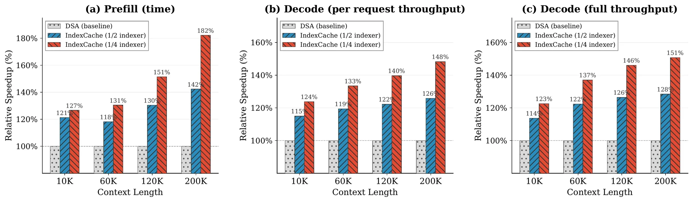
Figure from Bai et al. (2026), arXiv:2603.12201. Relative speedup of IndexCache over the DSA baseline (=100%) on the 30B model across prefill latency, per-request decode, and full decode throughput. Gains grow with context length.
On a 30B DSA model served in SGLang on an H100 node, deleting 75% of the indexers (1/4 retention) yields, at 200K tokens:
| Context | Config | Prefill (s) ↓ | Decode/req (tok/s) ↑ | Decode full (tok/s) ↑ |
|---|---|---|---|---|
| 200K | DSA baseline | 19.5 | 58.0 | 197 |
| 200K | IndexCache 1/2 | 13.7 | 73.0 | 253 |
| 200K | IndexCache 1/4 | 10.7 | 86.0 | 297 |
That’s 1.82× prefill and 1.48× decode at 200K — and the advantage only widens as context grows toward 1M, which is exactly the regime GLM-5.2 targets. The paper’s preliminary runs on the production 744B GLM-5 confirm it scales:
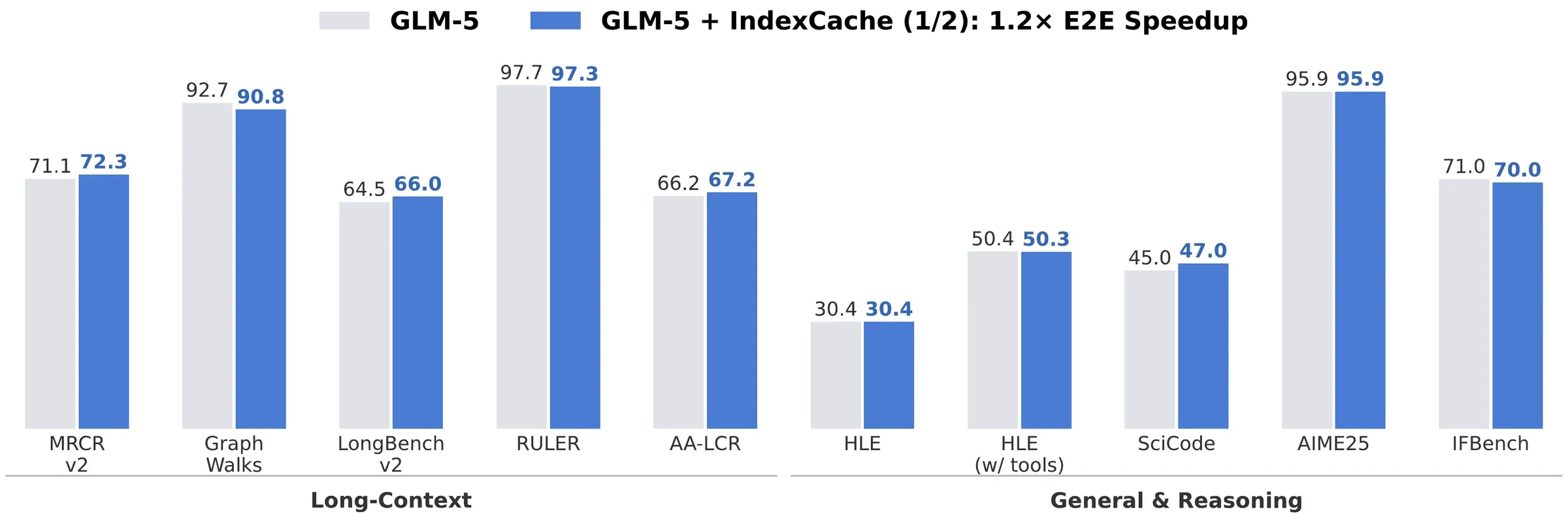
Figure 1 from Bai et al. (2026), arXiv:2603.12201. GLM-5 vs GLM-5 + IndexCache. Removing 50% of indexer computations holds long-context and reasoning quality while delivering ~1.2–1.3× end-to-end speedup at production scale.
KVShare + rejection sampling + the end-to-end TV loss
The second pillar is GLM-5.2’s rebuilt Multi-Token Prediction (MTP) stack for speculative decoding. This is where IndexShare, KVShare, rejection sampling, and the end-to-end TV loss combine — and the cleanest way to motivate them is to first see why naïve MTP gets slow exactly when you need it most: during RL.
MTP and the entropy bound
In MTP speculative decoding, lightweight draft heads propose candidate tokens with distribution , and the target model verifies them in a single forward pass with distribution . The expected number of tokens accepted per step — the thing you want to maximize — is
The Bebop paper (Qwen team) asks whether MTP can accelerate RL training — where rollouts dominate end-to-end time — and finds a nasty obstacle: the acceptance rate is fundamentally bounded by the target model’s entropy, and RL deliberately raises entropy to encourage exploration. The two factors usually blamed (draft/target distribution mismatch from weight updates) turn out to be secondary; the dominant driver is the entropy fluctuation .
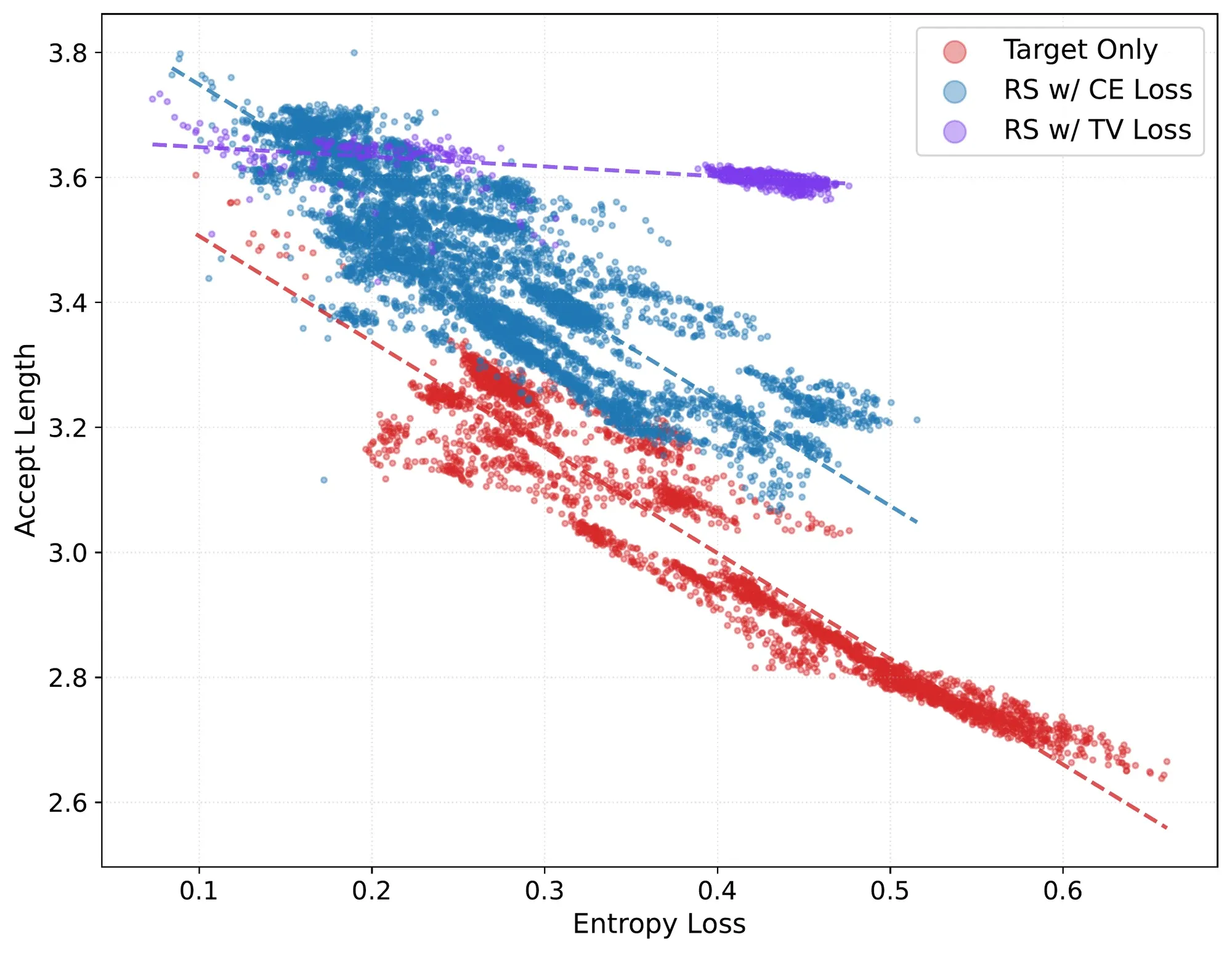
Figure 1(a) from Li et al. (2026), arXiv:2606.12370. Each point is the mean entropy and accept length at one RL step across Qwen3.5/3.6/3.7 runs. Target-only acceptance degrades linearly with policy entropy; rejection sampling + the e2e TV loss largely removes the entropy dependence.
Why does entropy bite? It depends on how you verify.
Target-only (greedy) sampling. Pick the draft’s and accept it with the target’s probability there. For a well-trained draft this gives
which is monotonically decreasing in — by Jensen, — and empirically near-linear,
So as RL pushes entropy up, greedy acceptance falls off a cliff.
Probabilistic rejection sampling. Draw and accept with probability . The expected acceptance rate is the full distributional overlap:
where is the Total Variation distance. This is unbiased (the output distribution is exactly , regardless of draft quality) and — crucially — it is governed by how well overlaps , not by how peaked is. That decouples it from entropy. So swapping greedy verification for rejection sampling is step one, and it’s already a large win in the high-entropy RL regime.
Why CE/KL is the wrong training loss here
If acceptance under rejection sampling is , then you should train the draft to minimize TV distance. But conventional MTP heads are trained with cross-entropy / forward-KL, . By Pinsker’s inequality,
KL is only a loose upper bound on TV — minimizing it doesn’t efficiently minimize the quantity that actually sets your acceptance rate. The gradient structure makes the difference concrete. CE/KL has gradient : a uniform per-token mismatch that spends optimization budget on the entire vocabulary, including the irrelevant long tail. That uniform mismatch accumulates over an effective support of size — which is precisely why CE-trained acceptance also ends up entropy-dependent.
The TV loss and its end-to-end form
So train against TV directly. The single-step TV loss is
with detached. Its gradient is
which is proportional to — it concentrates updates on tokens the draft already cares about and ignores the tail. This produces a probability-proportional mismatch instead of a uniform one, and that’s what decouples acceptance from entropy. It’s also a bounded gradient (), unlike KL’s which can blow up when and disagree — so it trains more stably.
Now the “end-to-end” part. Acceptance length is a product of per-step rates , so optimizing the average single-step TV distance ignores the multiplicative structure (early-step errors kill every downstream term). Bebop’s end-to-end (e2e) TV loss optimizes the normalized expected acceptance length directly:
Because each appears in every product term , earlier steps are weighted more heavily — and since the depend on current draft quality, it’s effectively a dynamic step-weighting that automatically shifts emphasis to whichever step is currently bottlenecking acceptance. No hand-tuned per-head loss weights.
Here is the whole thing in PyTorch — it’s strikingly small:
import torch
import torch.nn.functional as F

def tv_distance(p, q):
    # p, q: [..., V] probability distributions; p is detached (target)
    # d_TV = 1 - sum_v min(p, q)
    return 1.0 - torch.minimum(p, q).sum(dim=-1)

def e2e_tv_loss(target_logits, draft_logits_per_step):
    """
    target_logits: [B, T, V]                      -- target model, detached
    draft_logits_per_step: list of gamma tensors  -- one [B, T, V] per MTP head
    Returns the end-to-end (normalized expected accept-length) TV loss.
    """
    p = F.softmax(target_logits, dim=-1).detach()       # stop-grad through target
    gamma = len(draft_logits_per_step)

    alphas = []                                          # per-step accept rate alpha_i
    for q_logits in draft_logits_per_step:
        q = F.softmax(q_logits, dim=-1)
        alphas.append(1.0 - tv_distance(p, q))           # alpha_i = 1 - d_TV(p_i, q_i)

    # expected normalized accept length = (1/gamma) * sum_j prod_{i<=j} alpha_i
    cum, acc = 1.0, 0.0
    for j in range(gamma):
        cum = cum * alphas[j]                            # prod_{i=1..j} alpha_i
        acc = acc + cum
    return 1.0 - acc / gamma                             # minimize -> maximize E[L]
One practical wrinkle Bebop flags: the TV
min(p, q)is a full-vocabulary operation, and truncating it to a top- to save memory backfires — small causes loss spikes and instability, and even converges slower than the full-vocab loss. Pay for the full softmax here.
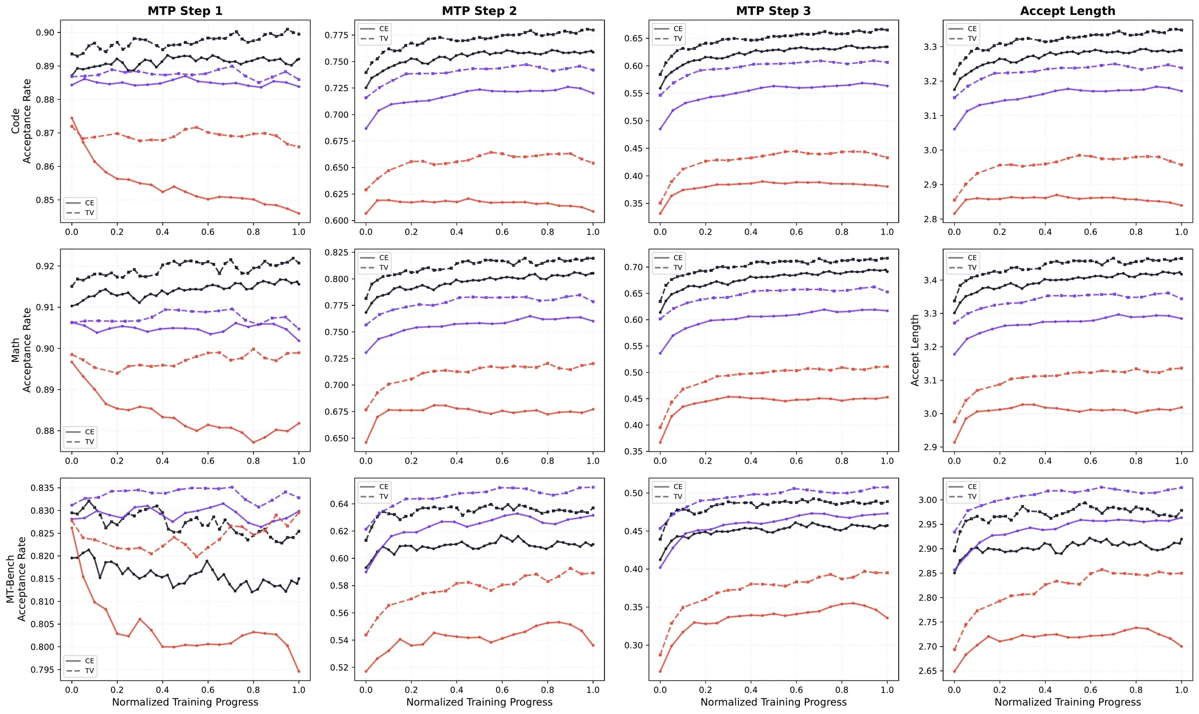
Figure from Li et al. (2026), arXiv:2606.12370. CE loss (solid) vs e2e TV loss (dashed) over SFT training; TV achieves higher acceptance at every MTP step, with the largest gains on later steps and agentic tasks.
On Qwen3.5-35A3B with , switching CE→e2e TV lifts rejection-sampling acceptance across the board:
| MTP loss | Math | Code | SWE | Agent | MT-Bench |
|---|---|---|---|---|---|
| CE (baseline) | 75.0 | 71.3 | 75.1 | 90.3 | 65.3 |
| e2e TV (ours) | +3.0 | +3.3 | +8.0 | +6.7 | +2.3 |
and the absolute numbers climb to up to ~95%+ at scale (e.g. Qwen3.6-Plus hits 99.1 on Agent). End to end, Bebop reports up to 25% extra inference throughput and 1.5–1.8× faster RL training (up to 2.4× on agentic RL), purely from a lightweight pre-RL MTP training phase — no MTP co-training during RL needed.
KVShare: closing the train/inference gap in GLM-5.2’s MTP
GLM-5.2 productizes all of this and adds KVShare, plus applies IndexShare to the MTP module itself. Two design choices matter:
- KVShare. In GLM-5.1 the MTP module’s KV cache was populated from mixed sources; in GLM-5.2 the MTP KV cache holds only the hidden states of the target model. The draft head therefore verifies against exactly the representation the target produces, eliminating a train/inference distribution gap that was quietly suppressing acceptance.
- IndexShare on MTP. The indexer is placed on the first MTP step, and its top- indices are reused for all subsequent draft steps — the same cross-layer trick, now applied across draft steps, so the draft heads stay cheap.
The ablation (acceptance length, higher is better) shows each piece compounding:
| Configuration | Acceptance length |
|---|---|
| Baseline | 4.56 |
| + IndexShare + KVShare | 5.10 |
| + Rejection Sampling | 5.29 |
| + End-to-end TV loss | 5.47 (+20%) |
That +20% acceptance length is the headline MTP number in the GLM-5.2 blog, and you can read off exactly where it comes from: KVShare/IndexShare make the draft consistent and cheap, rejection sampling makes verification entropy-robust, and the e2e TV loss trains the draft to maximize the quantity rejection sampling actually rewards.
Training: slime, OPD merging, and long-horizon RL
GLM-5.2 is built for long-horizon agentic work, and the post-training stack is organized around that goal, on Zhipu’s open-source slime RL framework.
Expert merging via parallel OPD. Rather than training one monolith, the team trained more than ten expert models (each strong in a domain) and merged them into the final model with parallel On-Policy Distillation (OPD) — the whole merge took ~2 days. OPD is the dense, on-policy distillation objective (roll out from the student, supervise toward an expert teacher with a per-token reverse-KL); if you want the theory of why it’s so sample-efficient versus RL, see the OPD-vs-RL post. slime exposes the rollout interface needed for this: white-box and black-box rollout, compact trajectory (trajectory compaction for long episodes), and sub-agent workflow modes.
Critic-based PPO for long horizons. Group-relative methods (GRPO and friends) assume comparable, similar-length rollouts in a group — which breaks down once trajectory compaction produces variable-length fragments. GLM-5.2 shifts to a critic-based PPO formulation: learn from individual rollouts and use a learned critic for token-level advantage estimation, which handles ragged, compacted long-horizon traces that group-wise baselines can’t.
Online anti-hacking. Long-horizon agentic RL is fertile ground for reward hacking (e.g. an agent that games the verifier rather than solving the task). GLM-5.2 runs a two-stage guard: a fast rule-based filter flags candidate hacks, then an LLM judge checks intent. Detected actions are blocked online while the rollout continues — so a single hacked action doesn’t poison the trajectory or destabilize training, and you don’t have to throw the whole rollout away.
Serving the 1M context. On the inference side, beyond IndexShare the engine adds finer-grained memory management and parallelism built on LayerSplit, kernel optimizations for context-dependent operations, and CPU-side cache management — and the throughput advantage grows as context length increases, which is the right shape for a 1M-token model.
Benchmarks
The full comparison from the GLM-5.2 release (bold = best open weight where applicable; * denotes figures reported with tools/caveats in the original table):
| Benchmark | GLM-5.2 | GLM-5.1 | Qwen3.7-Max | MiniMax M3 | DeepSeek-V4-Pro | Claude Opus 4.8 | GPT-5.5 | Gemini 3.1 Pro |
|---|---|---|---|---|---|---|---|---|
| HLE | 40.5 | 31 | 41.4 | 37 | 37.7 | 49.8* | 41.4* | 45 |
| HLE (w/ Tools) | 54.7 | 52.3 | 53.5 | — | 48.2 | 57.9* | 52.2* | 51.4* |
| CritPt | 16.7 | 4.6 | 13.4 | 3.7 | 12.9 | 20.9 | 27.1 | 17.7 |
| AIME 2026 | 99.2 | 95.3 | 97 | — | 94.6 | 95.7 | 98.3 | 98.2 |
| HMMT Nov. 2025 | 94.4 | 94 | 95 | 84.4 | 94.4 | 96.5 | 96.5 | 94.8 |
| HMMT Feb. 2026 | 92.5 | 82.6 | 97.1 | 84.4 | 95.2 | 96.7 | 96.7 | 87.3 |
| IMOAnswerBench | 91.0 | 83.8 | 90 | — | 89.8 | 83.5 | — | 81 |
| GPQA-Diamond | 91.2 | 86.2 | 90 | 93 | 90.1 | 93.6 | 93.6 | 94.3 |
| SWE-bench Pro | 62.1 | 58.4 | 60.6 | 59 | 55.4 | 69.2 | 58.6 | 54.2 |
| NL2Repo | 48.9 | 42.7 | 47.2 | 42.1 | 35.5 | 69.7 | 50.7 | 33.4 |
| DeepSWE | 46.2 | 18 | 18 | 20 | 8 | 58 | 70 | 10 |
| ProgramBench | 63.7 | 50.9 | — | — | 47.8 | 71.9 | 70.8 | 39.5 |
| Terminal Bench 2.1 (Terminus-2) | 81.0 | 63.5 | 75 | 65 | 64 | 85 | 84 | 74 |
| Terminal Bench 2.1 (Best Harness) | 82.7 | 69 | — | — | — | 78.9 | 83.4 | 70.7 |
| FrontierSWE (Dominance) | 74.4 | 30.5 | — | — | 29.0 | 75.1 | 72.6 | 39.6 |
| PostTrainBench | 34.3 | 20.1 | — | — | — | 37.2 | 28.4 | 21.6 |
| SWE-Marathon | 13.0 | 1.0 | — | — | — | 26.0 | 12.0 | 4.0 |
| MCP-Atlas (Public) | 76.8 | 71.8 | 76.4 | 74.2 | 73.6 | 77.8 | 75.3 | 69.2 |
| Tool-Decathlon | 48.2 | 40.7 | — | — | 52.8 | 59.9 | 55.6 | 48.8 |
The story the table tells: GLM-5.2 is at or near the closed-source frontier on math (AIME 2026 99.2) and competitive on agentic coding (Terminal Bench 2.1 81.0, FrontierSWE 74.4 — a 2.4× jump over GLM-5.1’s 30.5), trailing Claude Opus 4.8 on the hardest SWE marathons but doing so as an open-weight MIT model at a fraction of the serving cost. The generation-over-generation deltas (e.g. DeepSWE 18→46.2, SWE-Marathon 1.0→13.0) are where the long-horizon RL stack shows up.
Takeaways
GLM-5.2’s three innovations rhyme: each one identifies a quantity that was being recomputed or mis-optimized, and fixes it at the source.
- IndexShare notices the sparse-attention indexer was redundantly re-deciding the same top- in every layer, and shares it across layers — fewer per-token FLOPs at 1M context, validated up to 744B.
- Rejection sampling + the e2e TV loss notice that MTP acceptance was being capped by entropy and trained against the wrong divergence (KL instead of TV) — fixing both makes speculative decoding survive the high-entropy RL regime, and is what lets MTP accelerate RL training rather than just inference.
- KVShare notices the MTP draft was verifying against a slightly-wrong representation, and feeds it the target’s own hidden states.
Put together — and wrapped in slime’s OPD merging, critic-based PPO, and online anti-hacking — they’re why a 753B open-weight model can serve a stable, cheap 1M-token context and top the agentic-coding leaderboards. The weights and the two companion papers are all public, which is the best part: you can read exactly how it was done.
Sources. GLM-5.2 technical blog (Z.ai) · IndexCache, arXiv:2603.12201 · Bebop / e2e TV loss, arXiv:2606.12370 · GLM-5.2 weights on Hugging Face