Long-context attention is the bottleneck that every serious open-weight LLM has had to confront, and two of the most-discussed answers from 2024–2026 come from opposite directions. DeepSeek’s Multi-head Latent Attention (MLA), introduced in DeepSeek-V2 (arXiv:2405.04434) and carried forward in V3 and V3.2, keeps every layer globally attentive but rewrites the KV representation so the cache shrinks by an order of magnitude. Xiaomi’s hybrid attention, used in MiMo-V2-Flash (arXiv:2601.02780), keeps the per-layer attention pattern simple but stops doing global attention in most layers — five sliding-window layers interleaved with one global layer, repeated.
Both designs cut the long-context cost of vanilla multi-head attention by roughly the same factor. They get there by changing entirely different things, and the design surface those changes open up is what makes the two architectures interesting to compare. This post walks the math of each, lays out the architectural trade-offs, and looks at the infrastructure consequences — what each design forces (or saves) for training, inference, and KV cache management.
Table of contents
Open Table of contents
The shared problem
Standard multi-head attention costs in compute and writes floats of KV cache per layer. Both costs become limiting before the model gets interesting at frontier context lengths:
- Pretraining at already spends a sizable fraction of FLOPs in attention rather than FFN.
- Decoding is memory-bandwidth-bound: the GPU’s job is to stream every token’s KV cache through SRAM each step, and at that traffic dominates per-token latency.
- Serving wants large batches to amortize the FFN. KV cache per request kills batch size — a 70B-class model with full MHA at can spend tens of GB per request on KV.
The two ways out are obvious in retrospect: shrink the per-token cache (MLA’s bet), or skip most of the pairs (hybrid attention’s bet). Each comes with second-order consequences, and that’s where the interesting tradeoffs live.
Part 1 — Multi-head Latent Attention (MLA)
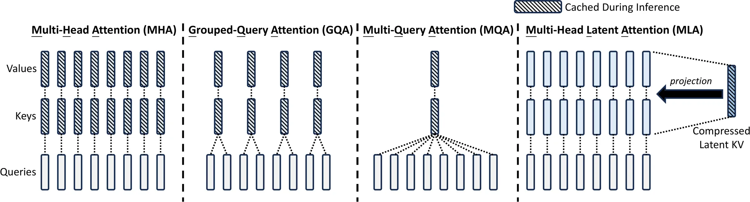
Figure 3 from DeepSeek-AI (2024), arXiv:2405.04434. MHA caches per-head K/V; GQA shares K/V across query groups; MQA shares one K/V across all heads; MLA caches a single low-rank latent per token (plus a small decoupled RoPE key), and reconstructs per-head K/V at compute time.
Setup
Let be the model hidden size, the number of heads, the per-head dimension. In standard MHA, the per-token KV cache for one layer is floats (the per-head and vectors). GQA collapses this to by sharing K/V across groups; MQA collapses further to with one shared K/V. The capability/cache tradeoff is well-known: MHA strongest, MQA weakest, GQA in between.
MLA’s promise is to beat MHA on capability while needing less cache than GQA. It does this with low-rank joint compression of K and V, plus a careful trick for RoPE.
Low-rank joint KV compression
The per-token hidden state is projected down to a small latent vector
The per-head keys and values are then reconstructed from this latent at use-time:
This looks like it just inserted a bottleneck. The non-obvious move is what gets cached. Only is written to the KV cache — the reconstructed and live only inside the attention kernel of the current step. The cache per token is floats instead of .
Querying is symmetric: queries also get a low-rank factorization, mostly to cut activation memory rather than cache,
The matrix-absorption trick
There’s a beautiful piece of algebra hiding here that makes MLA fast at inference. The reconstruction appears inside a dot product . Matrix multiplication is associative, so can be precomputed once per query step, and the per-token attention becomes a dot product directly against the latent .
Equivalently: can be absorbed into , and into the output projection , so at inference time the model never materializes per-head or . It attends directly to the latent cache, with no decompression cost on the prefix.
This is what makes MLA’s “MHA-level quality at sub-GQA cache” claim hold up in practice. Without the absorption, the model would have to multiply every cached latent by during decode, adding back the FLOPs the compression saved.
The RoPE problem and decoupled RoPE
Rotary position embedding (RoPE) is applied as a position-dependent rotation matrix to and before the dot product. If you apply RoPE directly to the reconstructed , the position rotation sits between and . Matrix multiplication is associative but not commutative — a position-dependent matrix cannot move past , so the absorption trick fails. You would be forced to re-derive from for every prefix token at every decoding step, which is exactly the cost MLA was supposed to avoid.
The fix is decoupled RoPE. Alongside the low-rank, RoPE-free and , MLA carries a separate small RoPE-bearing pair:
These have a small per-head dimension (DeepSeek-V2 uses alongside ). The full per-head query and key are concatenations,
with shared across all heads (so the RoPE path is effectively MQA-shaped while the content path is MHA-shaped). The attention dot product splits cleanly into a position-free term that participates in the absorption trick, and a position-aware term that is small enough that recomputing it from would be expensive anyway, so it is cached directly.
The cache per token becomes floats. In DeepSeek-V2, and , against an that full MHA would cache (per layer). That is a roughly 28× reduction. The paper notes this is equivalent to GQA at 2.25 groups, while quality slightly exceeds full MHA.
What the full computation looks like
Every layer attends globally to the entire prefix. The per-pair cost is the same as MHA (it’s still a softmax-weighted dot product), and the per-pair count is still per query. MLA does not reduce attention FLOPs; it reduces the memory footprint and bandwidth of the KV cache. Because decode is memory-bandwidth-bound, that translates almost directly into decode throughput.
Part 2 — Hybrid attention in MiMo-V2-Flash
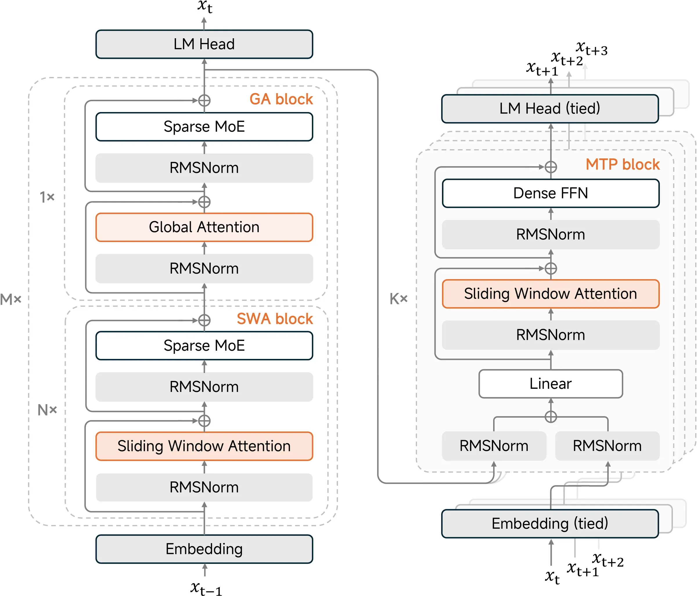
Figure 1 from MiMo-V2-Flash Technical Report, arXiv:2601.02780. Eight Hybrid Blocks, each five SWA layers followed by one Global Attention layer. The very first transformer block is a Global Attention layer with a dense FFN, for early-representation stability. MTP draft heads use SWA with a dense FFN.
The shape of the stack
MiMo-V2-Flash’s bet is structural rather than algebraic. Within each layer the attention is plain GQA softmax — no low-rank latent, no absorption trick. But most layers don’t see the full sequence. The 48 transformer blocks are organized as hybrid blocks, each consisting of Sliding Window Attention (SWA) layers followed by one Global Attention (GA) layer. The first transformer block is an exception: it uses GA with a dense FFN to stabilize early representations. The remaining 47 layers use the sparse MoE FFN (256 experts, 8 activated).
The headline numbers:
- Sliding window size tokens. Each SWA layer’s attention is masked to a band of width around the query position.
- SWA-to-GA ratio of 5:1. Of the 48 layers, 39 are SWA and 9 are GA.
- Roughly 6× reduction in KV-cache storage and attention compute for long contexts, since only 1/6 of layers have to maintain or stream a full-length cache.
Sliding window attention and why W = 128 is so small
Sliding window attention restricts each query at position to attend to keys in . The KV cache for an SWA layer is bounded by regardless of sequence length, and the per-token attention work is instead of . With this is essentially constant in .
The catch is that is aggressive. Earlier hybrid-attention models (Gemma 2, MiniMax-01) used larger windows in the 512–4096 range. MiMo’s ablation actually finds that a smaller window is better for long-context retrieval after long-context extension, which seems counterintuitive. Their interpretation: a tight window forces a clean division of labor. SWA layers handle local syntax and short-range dependencies; GA layers handle everything that has to span more than tokens. With the SWA layers can partially do long-range work, which dilutes both responsibilities and hurts the model’s ability to use the global layers efficiently.
The numerical receipt, from MiMo’s ablation: at with attention sinks (see below), hybrid SWA matches or beats all-GA on general benchmarks, beats it on long-context (RULER-32k, MRCR, NoLiMa), and beats it on hard reasoning (AIME, LiveCodeBench, GPQA). At , the long-context numbers collapse.
Attention sinks: the trick that makes aggressive SWA work
Naive SWA with very small has a well-documented failure mode: the softmax is forced to allocate attention mass even when nothing in the window is relevant, and at small this happens often enough to hurt quality. The standard fix, attention sink bias, lets each head learn a scalar that participates only in the softmax denominator:
The numerator stays a sum over the actual keys in the window. The denominator gets an extra term, the sink. If no key in the window is salient, the head can route most of the softmax mass to the sink, which contributes nothing to the output (the sink has no value vector) — effectively letting the head output near-zero when its window contains nothing useful, instead of being forced to mix in noise. MiMo’s ablation shows that without the sink bias, degrades MMLU and BBH by 2–3 points; with it, matches or beats all-GA across the board.
This is conceptually a learned “do nothing” option, and it’s the piece that lets the SWA:GA ratio be pushed to 5:1 without breaking the model.
What the GA layers do (and what they don’t)
The 9 global-attention layers in MiMo-V2-Flash are the only path by which information from outside a 128-token window reaches each token. They are full softmax attention with GQA (64 query heads, 4 KV heads, per-head Q/K dim 192, V dim 128). Because they are global, they remain in compute and in cache per GA layer — but there are only 9 of them, so the total long-context cost is ~9/48 ≈ 1/5 of all-GA, before counting the negligible cost of the SWA layers.
A consequence worth internalizing: the model’s ability to retrieve at long context lives almost entirely in those 9 layers. The SWA layers can be aggressively memory-tight because they aren’t doing the retrieval work; they just need to keep the local representation clean. MiMo reports near-100% retrieval accuracy from 32k to 256k, which is the empirical evidence that 9 GA layers is enough.
Part 3 — Side by side
| Question | MLA (DeepSeek) | Hybrid SWA (MiMo-V2-Flash) |
|---|---|---|
| Where does the saving come from? | Compress KV per-token via low-rank latent | Skip most KV pairs in most layers |
| Per-token cache | floats/layer (V2) | per SWA layer, full prefix per GA layer |
| Attention compute | Unchanged from MHA, in every layer | per SWA layer; only in GA layers |
| Per-pair work | Slightly cheaper than MHA after absorption | Standard softmax dot product |
| Position encoding | Decoupled RoPE (a small extra path) | RoPE on first 64 dims of Q/K, vanilla |
| What is uniform across layers? | The attention recipe — every layer is MLA | The block structure — every block is 5×SWA + 1×GA |
| Quality regime | Equal or slightly better than MHA | Equal or slightly better than all-GA, if attention sinks are used |
| Fragile points | RoPE incompatibility forces decoupled-RoPE plumbing | Without sinks, small-window SWA degrades; ratio/window must be tuned |
| Long-context retrieval | Lives in every layer | Lives in the GA layers |
The two designs occupy almost orthogonal points in the design space. MLA changes the K/V representation while keeping the attention pattern dense. Hybrid SWA changes the attention pattern while keeping the K/V representation simple. They aren’t even mutually exclusive — there’s nothing stopping a future model from running MLA inside the GA layers of a hybrid stack, and that would compound the savings — but neither MiMo nor DeepSeek has shipped that combination publicly.
What this means for KV cache at long context
A back-of-the-envelope for , in floats per request per layer:
- MHA, 64 heads × 128 dim: (per layer)
- GQA-8: per layer
- MLA, : per layer — applies to every layer.
- Hybrid SWA layer, , KV-heads = 8, dim = 128: per layer — applies to 5/6 of layers.
- Hybrid GA layer, KV-heads = 4, dim = 128: per layer — applies to 1/6 of layers.
Averaged over a 48-layer stack the hybrid model spends roughly floats per layer per request at — i.e. a smaller per-layer footprint than MLA. The catch is that the cost is unevenly distributed: the GA layers each carry the full 128k cache, and they are exactly the layers a serving system has to plan around. MLA’s footprint is large compared to a single SWA layer but uniform across the whole stack, which is easier to schedule.
Part 4 — Multi-Token Prediction, and how each architecture shapes it
Both DeepSeek-V3 and MiMo-V2-Flash ship with Multi-Token Prediction (MTP) modules, and both papers explain the motivation in the same terms — denser training signal, and a “free” speculative-decoding draft model at inference. What is less obvious until you read them side by side is that the MTP design in each model is heavily shaped by the upstream attention choice. MLA’s per-token-cache savings make MTP a parameter problem; hybrid attention’s per-layer pattern savings make MTP an attention-pattern problem. They end up at different points on the “how lightweight should the draft be” axis.
What MTP is, in one paragraph
Standard LM training predicts the next token at each position. MTP extends this so each position predicts the next tokens. At inference, the same modules can be repurposed as a draft model: the main model verifies the draft’s candidates in a single forward pass, and accepted tokens count as free output. Verification is cheap because it’s a single batched forward of the main model — the draft only has to be right often enough that average accept length is large compared to its overhead. The training-time and inference-time uses are largely independent: the training objective sharpens representations even if you never use MTP at inference; the inference draft works even if MTP wasn’t trained from scratch (you can attach MTP heads in a short post-training stage).
DeepSeek-V3’s MTP design
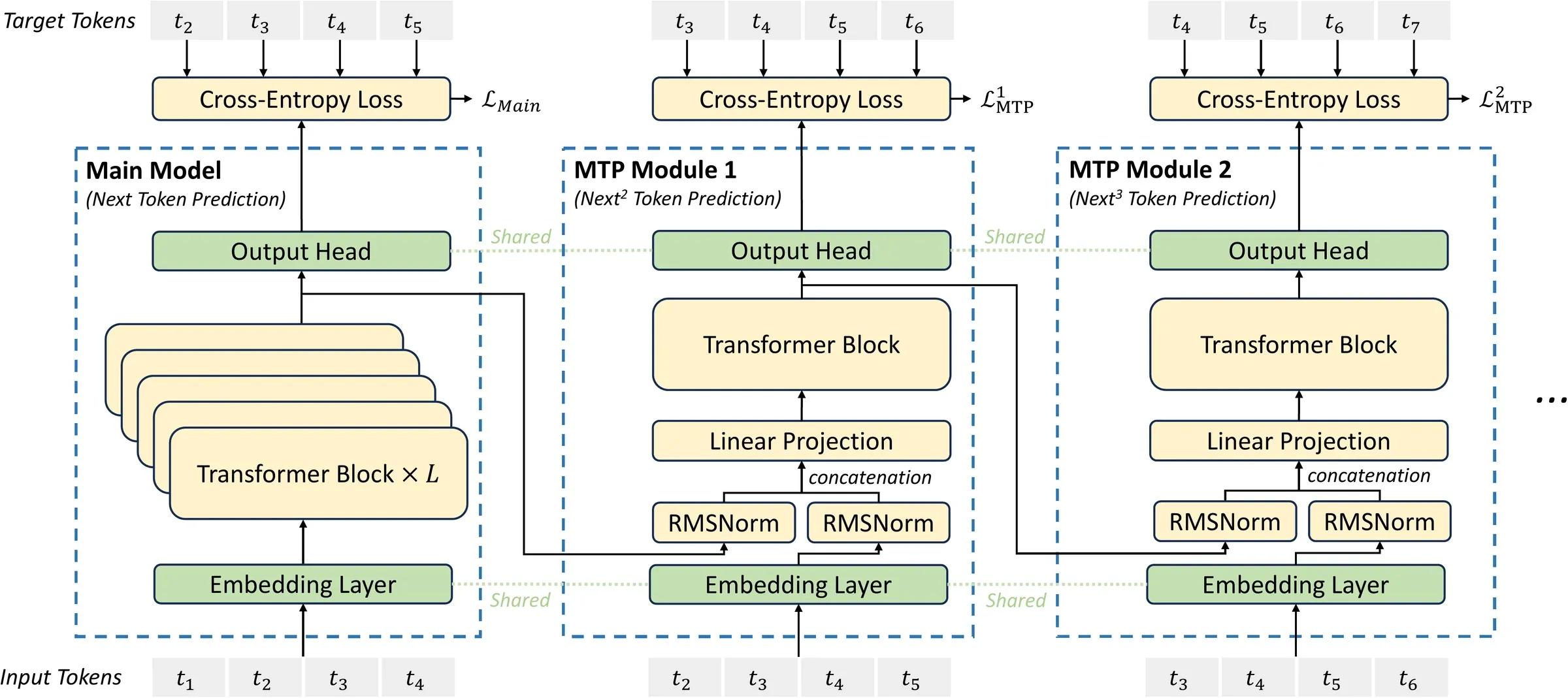
Figure 3 from DeepSeek-V3 Technical Report, arXiv:2412.19437. Each MTP module is a full Transformer block; embedding and output head are shared with the main model; the causal chain is preserved across depths.
The V3 implementation uses sequential MTP modules. Each module takes the previous module’s hidden state and the embedding of the future token , combines them with a linear projection , runs a full Transformer block, and produces a prediction through the shared output head:
A few details matter:
- Embedding and output head are shared with the main model, so the per-module parameter cost is one Transformer block plus the projection . At V3 scale that block is not small (full MoE FFN, full MLA attention), but it’s still a few percent of total parameters per MTP head.
- Sequential, not parallel. Meta’s original MTP proposal predicts tokens in parallel with independent heads from one hidden state. V3 keeps a causal chain: the head predicting token has consumed the hidden state that predicted token . This makes the draft chain more coherent — token-’s prediction is conditioned on token-’s representation — at the cost of sequential Transformer evaluations per step in the draft.
- Training loss. Per-depth cross-entropy, averaged across depths, with a weight on the combined loss. V3 sets for the first 10T tokens of pretraining and for the remaining 4.8T. Empirically the MTP objective improves the main model’s evals even when the MTP modules are discarded at inference.
- Inference. The MTP modules can either be discarded (the main model still works fine — it was the primary target) or repurposed as the draft for self-speculative decoding.
Because each V3 MTP head is itself a full Transformer block, the draft is not what you’d call lightweight. It runs MLA attention (with its own KV cache!) and MoE FFN, same as the main model. The speedup story is more about parallelizing verification than about a cheap draft: the main model verifies tokens in one pass instead of passes, so even a moderately accurate draft pays.
MiMo-V2-Flash’s MTP design
MiMo takes the opposite philosophy. The MTP block is “deliberately kept lightweight to prevent it from becoming a new inference bottleneck.” Two ablations from the main architecture are dropped in the draft:
- Dense FFN instead of MoE. The main model’s 256-expert / 8-active MoE FFN is replaced with a small dense FFN in the MTP block.
- SWA instead of GA. The MTP block uses sliding-window attention only. No global attention.
The result is an MTP block of 0.33B parameters — under 0.5% of the 309B-parameter main model and ~2% of the 15B active parameters. Compare this to a V3 MTP head, which is a full main-model layer.
The training recipe matches the lightweight design:
- During pretraining, a single MTP head is attached to the model — enough to densify the training signal without paying for heads of training compute.
- In post-training, that single head is replicated times and the -head stack is jointly trained for multi-step prediction. Each head receives both the main-model hidden state and the embedding of the next token, same as V3.
Because the draft is so much smaller than the main model, the draft cost is negligible in the speculative loop. The reported decoding speedups, with a 3-layer MTP stack on 16K input / 1K output:
| Per-node batch | w/o MTP | accept length 3.0 | 3.4 | 3.8 |
|---|---|---|---|---|
| 32 | 1.00× | 1.99× | 2.25× | 2.52× |
| 64 | 1.00× | 2.11× | 2.39× | 2.67× |
| 96 | 1.00× | 2.13× | 2.42× | 2.70× |
| 128 | 1.00× | 1.94× | 2.20× | 2.46× |
Empirically, accept length scales inversely with next-token cross-entropy: low-entropy contexts (e.g. WebDev autocomplete) reach ~3.6 accepted tokens per step; high-entropy contexts (MMLU Pro) bottom out near 2.8. MiMo fits this with , . The takeaway: MTP is most useful exactly when the model is most confident, which is fortunate — those are also the contexts (code, formatting, structured output) where decoding throughput matters most in practice.
Why the designs diverge — the architecture argument
The interesting observation is that the upstream attention design forces a different draft design.
For MLA, every layer is the same operator, and the KV cache per token is already small. There is no obvious knob to make a draft layer cheaper than a main-model layer: you can’t drop low-rank compression (then the cache balloons), and you can’t drop global attention (every MLA layer was already global by design). The savings have to come from elsewhere — either fewer MTP heads, lower weight on the MTP loss, or making the draft’s FFN/MoE smaller. V3 essentially says “the draft layer is a main-model layer; the savings come from parallel verification of tokens at once.” This is the natural move when your attention is already as cheap per token as you can make it.
For hybrid SWA, the SWA-vs-GA decision is the knob. The model has empirically shown that 5-of-6 layers can be SWA without hurting quality. That gives the architect a ready-made compression for the draft: build the MTP block out of only the cheap kind of layer — SWA only, dense FFN only, no MoE, no global attention. The draft inherits a smaller version of the same inductive bias. The MTP block is essentially the “what does a single hybrid-block step look like, minus everything expensive?” question made concrete.
This is the cleanest example in either paper of a cross-talk between the attention choice and a downstream design decision. MLA encourages a verification-parallel draft because it has nothing cheap to drop. Hybrid attention encourages a cheap-architecture draft because it has cheap layers ready to use. Different bets at the attention layer compound into different decisions a few abstraction levels up.
A small but important RL connection
One last MTP point that didn’t fit elsewhere. MiMo motivates MTP partly as an RL training accelerator. RL post-training (PPO, GRPO, and friends) spends most of its wall-time in the rollout phase — running the model in inference mode to generate trajectories. The rollout phase has two pathologies:
- Underutilized GPUs at small batch sizes. On-policy RL prefers small batches for stability, which leaves FFN arithmetic intensity low and KV cache traffic dominant.
- Long-tail stragglers. Different rollouts finish at different times; near the end, only a few sequences are still running at batch size ~1.
MTP fights both. It increases token-level parallelism (multiple drafted tokens per step) without increasing KV traffic, raising the effective arithmetic intensity. And on the long tail, where the batch has collapsed to a single sequence, MTP gives you a multiplicative speedup just when you need it most. The architectural choice (hybrid attention) and the training-stage choice (RL post-training) feed into each other here: the lightweight MTP block exists because the hybrid stack made it possible, and the lightweight MTP block makes the RL pipeline tractable.
Part 5 — Infrastructure implications
Architecture choices set the constraints that training and inference infra have to live with. Here’s what each design pushes onto the stack around it.
Training infrastructure
MLA’s training surface is conventional. Every layer is the same attention operator. Tensor-parallel sharding by heads works exactly as it does for MHA — the low-rank projections add some small matmuls but no new parallelism axis. The decoupled-RoPE path adds bookkeeping but no new communication primitive. MLA was designed alongside DeepSeek’s expert-parallel MoE stack and the two are largely independent: the attention savings cut activation memory and let DeepSeek-V2 be trained at 60 layers / 5120 hidden / 128 heads without tensor parallelism, which in turn simplifies the parallel mesh.
Hybrid attention adds heterogeneity. Five different layer shapes — SWA blocks with sparse MoE, GA blocks with sparse MoE, the special first block with GA + dense FFN, the SWA MTP blocks with dense FFN. A pipeline-parallel partitioning has to deal with two cost profiles per block (GA is meaningfully more expensive than SWA) which complicates load balancing across pipeline stages. Sliding-window kernels need their own attention masks and benefit from specialized kernels (e.g. FlashAttention’s local-attention variant). MiMo’s recipe deals with this empirically: they pre-train on 27T tokens with FP8 mixed precision, similar in shape to DeepSeek-V3.
Both models keep BF16 for attention output projection and FP32 for MoE routers — the FP8 mixed-precision recipe is closer to a shared playbook than a differentiator.
Inference infrastructure
MLA’s win is mostly on the prefill-and-decode pipeline. The cache per token is small and contiguous (one latent vector, plus a small RoPE key). Decode is memory-bandwidth-limited, so a 10–30× reduction in cache size translates directly into proportional throughput, larger batches, and longer context budgets per GPU. The matrix-absorption trick eliminates the prefix-K reconstruction cost. The price is two small extra GEMMs in the attention block (down-projection and up-projection on the active token’s queries), but those are tiny against the savings.
Hybrid attention’s win is mostly on the prefill side, with a different shape on decode. Prefill compute scales with where is the effective receptive field of layer ; for hybrid SWA that sum is , which at is dominated by the GA term but is still ~6× smaller than all-GA. Decode reads entries per SWA layer and entries per GA layer per step — most of the bandwidth is in the 9 GA layers, but those 9 are large and need to be served well.
The two implications are different enough that the serving stack tends to look different. MLA-friendly serving stacks (vLLM, SGLang with MLA support, DeepSeek’s reference implementations) optimize for uniform per-layer KV scheduling and for the absorption trick on the indexer path. Hybrid-attention serving stacks (gpt-oss, Gemma 2/3, MiMo) optimize for heterogeneous scheduling: SWA layers can flush their cache aggressively (no token beyond steps old is ever read again), while GA layers need the full long-context infrastructure.
Long-context extension
The “extend a model from 32k to 256k” pipeline interacts with each design differently:
- MLA has nothing position-specific in its compressed-attention path; only the small decoupled-RoPE path sees position. Extension recipes (YaRN, NTK-aware scaling) operate on that small path, which is cheap and well-understood.
- Hybrid SWA: the SWA layers don’t care about absolute position past , so extension is concentrated in the 9 GA layers. MiMo reports a clean extension from 32k native context to 256k, with near-100% retrieval across the range. The GA layers do all the work; the SWA layers don’t need to be retrained on long sequences.
Part 6 — What does the tradeoff actually buy
If you imagine the design space as a 2D plot — KV cache shrink on one axis and attention compute shrink on the other — MLA sits high on the cache axis with no compute reduction; hybrid SWA sits moderately on both. The honest summary is:
-
MLA is the safer architectural change. Every layer is the same operator; the change is upstream of how K and V are stored. You give up nothing in the attention pattern. The cost is plumbing (decoupled RoPE, absorption tricks at inference time) and a slight scale-up in attention-side parameters (the up-projection matrices). MLA is a good default for a dense or MoE model that wants to push context length without rethinking the layer recipe.
-
Hybrid attention is the bolder bet, and is more compute-efficient on prefill. Skipping most pairs in most layers is a much larger saving in raw FLOPs than compressing K/V. But it relies on attention sinks to make small windows work, requires careful ratio/window tuning, and creates heterogeneous compute and cache patterns that the infra stack has to live with. The reward is a model that scales gracefully to 256k+ context with near-constant decode cost in the SWA layers.
-
They are not competitors so much as complements. The DeepSeek-V3.2 paper (which retrofitted sparse attention onto an MLA-based stack) is the clearest existing example of layering one of these ideas on top of the other. A future model that runs MLA inside hybrid GA layers — full-rank globally rare, low-rank in those few global slots — would compound the savings in a natural way. We haven’t seen it ship publicly, but the design surface is wide open.
The deeper takeaway from reading the two papers back-to-back is that the constraints of the production stack often determine which trade looks attractive. DeepSeek started from an “every layer should look the same” worldview and re-engineered the K/V representation. Xiaomi started from a “small windows are cheap, attention sinks make them work” worldview and re-engineered the per-layer pattern. Either move is defensible. The interesting questions show up downstream — in how they shape MTP, FP8 quantization, KV serving, and long-context extension — and that’s where the architectures stop being interchangeable.
Closing
MLA and hybrid attention are two genuinely different answers to the same question, and that is rarer than it sounds. Most attention variants since 2022 have been minor tweaks on a shared template; MLA and hybrid SWA actually disagree about which axis to compress on. Reading them together is the cheapest way to internalize the modern design space — what you give up, what you keep, and what the rest of the stack has to do differently to make it pay off.
If you’ve made it this far and want to chase the thread further, the natural next stops are NSA and DSA (DeepSeek’s sparse attention designs, covered in this blog post) which sit on a third axis — sparsifying which pairs are computed inside each attention call — and the open question of whether a future model wants to combine all three.
References
- DeepSeek-AI. DeepSeek-V2: A Strong, Economical, and Efficient Mixture-of-Experts Language Model. arXiv:2405.04434, 2024.
- DeepSeek-AI. DeepSeek-V3 Technical Report. arXiv:2412.19437, 2024.
- LLM-Core, Xiaomi. MiMo-V2-Flash Technical Report. arXiv:2601.02780, 2026.
- Beltagy, I., Peters, M., Cohan, A. Longformer: The Long-Document Transformer. arXiv:2004.05150, 2020.
- Agarwal, A. et al. gpt-oss. (Attention sink bias formulation referenced by MiMo-V2-Flash.)